Physics-informed neural networks (PINN)
On this page
GIST 오현석 교수님 Recent Trend in PINN and its Applications to NDT
포항공대 최민석 교수님 Recent Advances in Physics-informed Machine Learning
강의 정리 내용입니다.
- Deep Learning
데이터가 충분하다면, domain knowledge 없이 잘 예측. → 하지만 데이터가 충분한 경우가 많던가?에 대한 의문.
왜 잘되는지 모름
일반화 문제. 주어진 데이터 안에선 결과가 잘 나오는데 조금만 바운더리 넘어가도 결과가 잘 안나오는 문제(extrapolation)
\(\Rightarrow\) Physics를 결합하여 해결해보자!
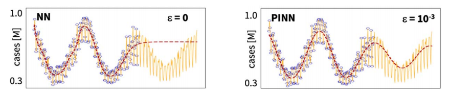
(우측, 2nd order differential equation을 추가한 PINN)
Linka et al., “Bayesian physics informed neural networks for real-world nonlinear dynamical systems”, CMAME, 2022.
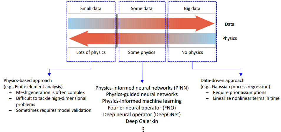
- 대부분의 경우, 중간처럼 some data + some physics 인 경우가 많음
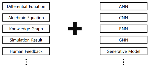
Physics Knowledge + Deep Learning Model
- 대부분의 연구는 Differential Equation + ANN
- Solving Differential Equations Using NN
Forward problem과 Inverse problem이 있다.
Forward는 differential equations를 푸는 문제,
Inverse는 differential equation의 unknown parameter(coefficient)를 추정하는 문제
- Physics-informed neural networks (2019)
No prior assumption - 가우시안이나 베이지안 접근법은 사전분포에 대한 assumption이 필요
No linearization - nonlinear가 심한 문제는 보통 linearization하고 푸는데 여기선 그럴 필요가 없다.
No local time-stepping - 계산비용이 많이드는데 PINN은 이 과정이 불필요하다.
- PINN Architecture
Artificial neural networks (ANN): universal function approximators
Given
Some data
Nonlinear PDEs
Minimize two losses(Data loss, PDE loss) during training
- PINN for Burger’s Equation
(Forward problem) Data-driven solution
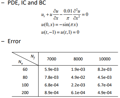
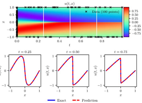
- PINN as a more accurate and computationally efficient “Surrogate Model”
(Inverse problem) Data-driven discovery
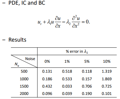
\(\lambda_1, \lambda_2\) 는 unknown, 추정하게 된다.
noise가 커도 좋은 효과를 보임
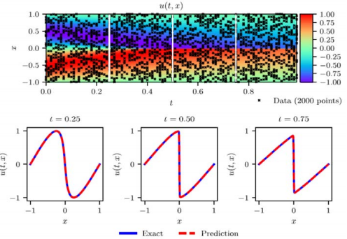
- PINN as a robust “system identifier” under scattered and noisy data
- PINN as a Numerical Solver
Benefits of PINN over conventional numerical solvers (e.g., FEM)
Works for ill-posed problems: noisy data, missing boundary conditions
Once trained, inference time is (at least) hundreds times faster.
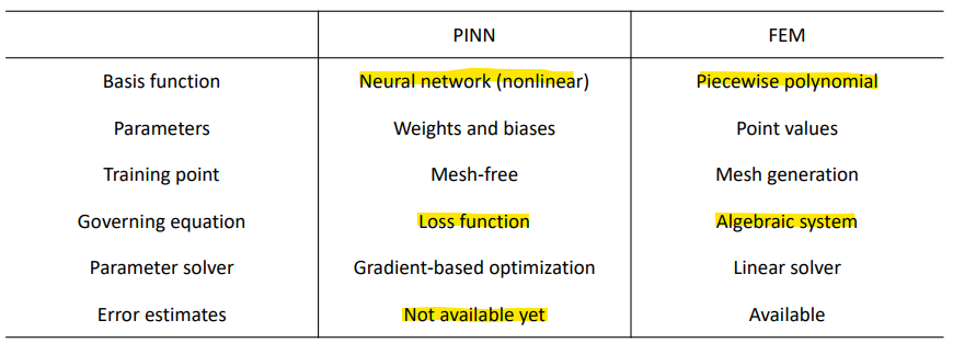
아직까지는 PINN이 error를 정확히 추정하는 것이 어려움
- Physics-informed Machine Learning (2021)

In the previous study by Raissi et al. (2019)
Some data
ANN only
Nonlinear PDEs
이 논문에선… Embedding physics into ML models extensively
Observational bias: e.g., multi-fidelity data
Inductive bias: e.g., CNNs, GNNs 다양한 아키텍쳐 사용 가능
Learning bias: e.g., PDEs
- Limitation of PINN: Single Instance Solver
Trainded PINN models predict only for a single instance
For given ICs, BCs, PDEs, the trained PINN models are effective. PDE의 coefficient들이 다 고정되어 있을 때, ICs, BCs가 고정되어있을 때 문제를 풀게된다.
- 이 값들이 바뀌면 처음부터 다시 학습을 시켜야한다. ex) 커피컵의 형상이 바뀌거나, 내용물이 꿀로 바뀌거나 등…
\(\Rightarrow\) Not very useful for most engineering problems.
- Neural Operator
앞의 내용을 극복하기 위한…
원래 PINN은 \(\mathbb{R}^{d_1} \rightarrow \mathbb{R}^{d_2}\) 다음과 같이 point to point
e.g., image classification
Operator는? function(\(\infty\) - dim) \(\rightarrow\) function(\(\infty\) - dim) function을 넣으면 function이 나옴. BC 등 이 바뀌더라도 결과가 바뀌어서 나온다.
e.g., derivative: \(x(t) \rightarrow x'(t)\)
e.g., integral: \(x(t) \rightarrow x\int K(s,t)x(s)ds\)
e.g., dynamic system: \(x(t) \rightarrow [\text{System}] \rightarrow y(t)\)
Mathematical backgrounds for NN operators are established in 1995. However, never be realized due to curse of dimensionality (i.e., Extremely expensive)
- Deep Operator Network (DeepONet; 2021)
- 실시간으로 앵글이 바뀌거나 해도 잘 작동한다.
- Multi-fidelity Data
In a particular problem,
A large amount of low-fidelity data
A small amount of high-fidelity data. 원래는 이걸로 학습시키는 경우가 많다. \(→\) 둘다 동시에 써보자!

Possible approach: incorporate multi-fidelity data into PINN or DeepONet
Low-fidelity training data는 경향성을 잘 보여주고
High-fidelity training data는 적은 양이지만 실제 값을 잘 추정한다.
이 둘을 결합했더니 exact 값을 잘 따라간다고 한다.
- Coefficient가 바뀌어도 잘 예측하는 모습을 보인다고 한다.
- Limitation of PINN: Convergence
PINN은 automatic differentiation을 사용하는데,
Universal approximation theory에 의해 continuous 는 잘 추정하지만 discontinuous와 singularity에선 문제가 발생한다.
Convergence depends largely on solution space.
- How to Improve?
Domain decomposition
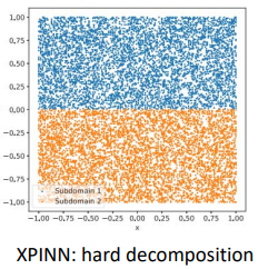
윗부분에 맞는 PINN과 아랫부분에 맞는 PINN을 만들어서 합치자!
- 중간부분에서 에러발생
cPINN (2020), XPINN (2020), FBPINN (2021)
Augmented PINN (APINNs) by Hu et al., EAAI (2023)
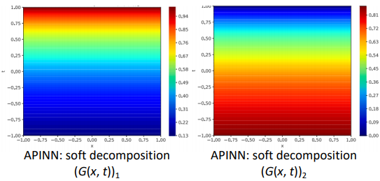
Soft domain decomposition
- weight를 줘서 2개의 PINN을 combination
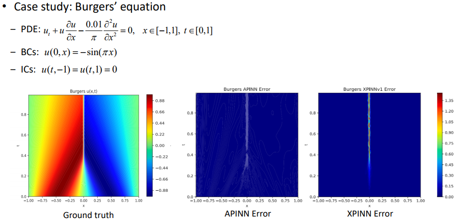
- 잘못 쓰여진 듯?? ICs와 BCs가 바뀜!! IC는 t=0 일 때!!(초기 시점)
- Nevertheless, Many Questions …
8 layers and 40 neurons를 썼는데 이게 최적?
Hundreds to thousands 데이터를 썼는데 이걸로 충분?
Adam, Quasi-Newton, or L-BFGS 등 다양한 옵티마이저 중에서 무엇이 최선?
…
- Research Issues in PINN
PINN is not perfect; fails for many problems using vanilla PINN.
Fundamental reasons behind this failure still remain unclear.
Long-time integration: often fails for transient problems
- Sequential learning으로 어느정도 해결 가능
Architecture design: best architecture for PINN? (e.g., CNN for computer vision)
Training dynamics: accelerating the training of PINNs?
- NTK를 이용해 PINN에서의 training dynamics를 어느정도 이해
Multiscale and multi-physics
- Fourier feature embedding이 spectral bias를 해결할 수 있다는 것이 알려져 있다.
Sampling method: How to distribute the collocation points and the corresponding weights?
sampling point 관련.. Uniform sampling → Importance sampling
Self-Adaptive PINNs - 각 point에 대해 weight를 준다.
Complex domains: domain decomposition strategies
And much more… lots of research opportunity !!
PINN 썼는데 잘 안될 때 추천 - Self Adaptive PINNs
- 오현석 교수님 연구 (Defect Detection by Ultrasonic Wave in NDT)
Unet + PDE loss만 썼을 때 결과가 잘 안나오더라..
→ random walk noise 추가, Loss function에 self-adaptation weights 추가, defect에 대한 위치를 또다른 Unet을 이용해서 인위적으로 집어넣어버림
→ 성능개선!
- Concluding Remark
- Extrapolation, generalization을 위해 물리지식을 적극 활용하자.
- Universal Approximation Theorem (Cybenko)
Let \(\sigma\) be any continuous sigmoidal function. Then, the superposition of the form
\[G(x) = \sum^N_{j=1} \alpha_j \sigma(y_j · x + \theta_j)\]
are dense in \(C(I).\)
Neural networks are good nonlinear approximators for function!
In fact, they are good approximators for operators as shown in [Chen].
Mathematical open questions:
How many neurons/layers?
How long is the optimization?
Does it overfit / generalize well?
High dimensional problem에서도 잘 작동한다.
- PINN Algorithm
Consider the deterministic PDE
\[u_t = \mathcal{N}(u), \quad x\in D, t \in [0, T].\]
주어진 PDE가 있을 때 exact solution은 구하기 어렵기에 근사하여 \(u(x,t)\) 를 찾고 싶은 것
universal approximation theorem에 의해 DNN의 아웃풋으로 근사를 하겠다.
\(\hat{u}(x,t;\theta)\) : surrogate of \(u(x,t)\) from DNN - 인공신경망으로 부터 오는 surrogate
\(\theta\) : DNN parameters. 최적의 파라미터를 찾는 것이 목표다.
\(\hat{u}\) from DNN should respect the given governing equation, i.e.
\[f(\hat{u}; \theta) := \hat{u}_t - \mathcal{N}(\hat{u}) \approx 0\]
constraint. residual을 봤을 때 정말 좋은 해라면 0에 가까워야 한다. → 최적화의, loss function의 constraint로 놓게 된다.
여기서
\(\hat{u}\) 는 신경망이 예측한 해(solution)
\(\hat{u}_t\) 는 \(\hat{u}\) 를 시간 \(t\) 에 대해 미분한 값, 시간 변화율을 나타내며 시간에 따라 변화하는 시스템의 특성을 설명한다.
\(\mathcal{N}(\hat{u})\) 는 \(\hat{u}\) 에 적용되는 미분 연산자(differential operator)
\(f(\hat{u};\theta)\) 는 PDE의 잔차(residual), 즉 좋은 해라면 0에 가까워야 함
Training data:
Initial and Boundary conditions: \(\{(x_{IB}^{(i)}, t_{IB}^{(i)}, u^{(i)})\}^{N_1}_{i=1}\)
PDE만 있으면 안되고 IC와 BC가 있어야 unique한 솔루션을 제공할 수 있다.
Collocation points for \(\mathcal{R}: \{(x_c^{(i)}, t_c^{(i)}, 0)\}^{N_2}_{i=1}\)
Residual에 대한, 도메인 내에서의 포인트
Loss function:
\[\mathcal{L}(\theta) = \frac{1}{N_1} \sum^{N_1}_{i=1}|\hat{u}(x_{IB}^{(i)},t^{(i)}_{IB})-u^{(i)}|^2 + \frac{1}{N_2}\sum^{N_2}_{i=1}|f(\hat{u}(x_c^{(i)}, t_c^{(i)}))|^2\]
앞부분은 IC, BC로 부터 오는 MSE, 뒷부분은 residual에서 오는 Error
뒷부분인 residual 계산부분 \(f(\hat{u}(x_c^{(i)}, t_c^{(i)}))^2\) 은 differential operator(automatic differentiation) 가 있기에
PDE는 미분을 계산해야 되는데 미분이 operator에 의해 정확히 계산 가능하다.
Train DNN to find the best parameters \(\theta^*\) by minimizing the loss function
\[\theta^* = \text{arg min} \mathcal{L}(\theta)\]
이후 loss function을 최소화하는 파라미터를 찾는 것이 PINN의 기본 아이디어.
The function \(\hat{u}^*(x,t;\theta^*)\) is approximate solution \(u\) of the given PDE.
[Prediction] Forward pass through NN with new input \((x,t)\) gives the solution \(u(x,t)\) .
최소화하는 파라미터를 찾았으면 그걸 통해 forward pass를 통하여 임의의 포인트 input x와 t에 대해 solution(prediction)을 찾아낼 수가 있는 것